Counting or summing vlookup in Excel or OpenOffice.org Calc
First published on January 14, 2010
Supposing you have a spreadsheet with keys (Domains) and values (Count):
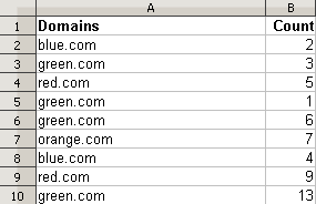
If you want to display the count for “orange.com” in a different cell, you would use the function VLOOKUP, whose basic use is nicely described here.
But as in the screenshot above, certain domains such as “green.com” appear several times. What if you wanted to sum the values of all of the “green.com” counts?
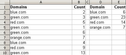
The solution doesn’t actually involve VLOOKUP, although it is somewhat in the spirit of VLOOKUP. Rather, you would use the function SUMPRODUCT, which multiples two columns and sums, well, the products. However, we only want to include certain rows if they match our criteria. This involves testing the key (Domain); the result of our test would be TRUE, which has a value of 1, or FALSE, which has a value of 0.
In E2 (replace comma with semi-colon for OpenOffice.org Calc):
=SUMPRODUCT($A$2:$A$10=D2,$B$2:$B$10)
In E3:
=SUMPRODUCT($A$2:$A$10=D3;$B$2:$B$10)
… and so on. E2 is essentially summing 1 * 2 and 1 * 4 for the blue.com rows and 0 * the count for all the other rows.
The actual spreadsheet I was working on involved full URLs containing the domain:
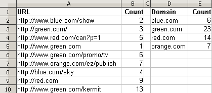
Therefore, I couldn’t do a simple comparison. I had to do something more like “does the URL contain a certain domain”. This is where the function SEARCH (case insensitive, as opposed to the case-sensitive function FIND) came in.
In E2 (replace the commas with semi-colons for OpenOffice.org Calc):
=SUMPRODUCT(ISNUMBER(SEARCH(D2,$A$2:$A$10)),$B$2:$B$10)
In E3:
=SUMPRODUCT(ISNUMBER(SEARCH(D3,$A$2:$A$10)),$B$2:$B$10)
… and so on.
Since the SEARCH function returns a number (specifically, the placement of the needle in the haystack) and the error “#VALUE!” if the search term does not exist, the ISNUMBER function will return 1 or TRUE when there’s a search match.
———————————
Limitations: If you’re doing something similar to this with URLs, note that we are searching for “blue.com”, “green.com” and so on to appear anywhere in the URL. You’ll need a more robust solution to support matching those strings only in the domain (since technically you could have a URL “blue.com/green.com”.
 Facebook
 Twitter
 Email this
 keung.biz. Hire my web consulting services at


February 16th, 2010 at 2:18 am
Aziyo says:
Good tips, Peter. In problem #1, For large datasets, INDEX & MATCH functions perform much quicker than an exact match VLOOKUP:
=INDEX($B$2:B10,MATCH(D2,$A$2:$A$10,0))
Once you get comfortable with them, you’ll never use a VLOOKUP again.
For the 2nd problem, SUMIF gets the same solutoin and may be easier to wrap your head around:
=SUMIF($A$2:$A$10,D2,$B$2:$B$10)
For #3, an array formula (CTRL-SHIFT-ENTER) using the same logic, but not easy to read:
{=SUM(IF(ISERROR(SEARCH(D2,$A$2:$A$10))=FALSE,$B$2:$B$10))}
Another option is to use a PivotTable with a helper column of String functions to isolate the domain name. This is faster for large datasets (or slow computers!) and doesn’t require re-typing domain names.
March 11th, 2010 at 2:22 am
Dave says:
Hi, thanks for your tips. Just thought you might like to know that (my version at least of) Excel doesn’t seem to cope with the first one (I haven’t tested the rest) because of an issue with the result’s format and just returns zero. So some extra brackets and forcing it to be a number-result with +0 helps it out.
Original:
=SUMPRODUCT($A$2:$A$10=D2,$B$2:$B$10)
Fixed for Excel:
=SUMPRODUCT(($A$2:$A$10=D2)+0,$B$2:$B$10)
November 21st, 2011 at 11:22 am
Lisa says:
I also had an issue with SUMPRODUCT in Excel 2010. Didn’t try Dave’s fixed option but did get solution with SUMIF. I was trying to sum debits when the transaction description was "Tx to Savings". Originally, VLOOKUP worked…the first time… but then duh…there was no instruction to sum. Removed vlookup and SUMIF worked great with *-1 of course to make the debit a positive number. Thanks for the inspiration!
=SUMIF(A2:A20,"Tx to Savings",B2:B20)*-1